A Brief Introduction to Deep Learning

Considering that the organizational structure under the Intelligenism framework, as discussed in later sections, will draw on the network structure of deep learning and incorporate some logic from reinforcement learning to enable organizations to exhibit intelligent features similar to those of intelligent programs, this section provides a brief introduction to deep learning. By understanding the network structure and working principles of deep learning through this section, readers can more easily grasp the subsequent content related to the settings and logic of the Intelligent Consortium.

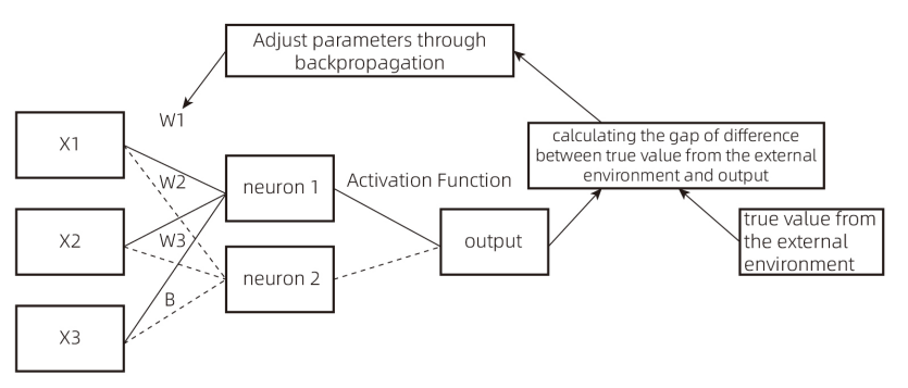
Figure 1

X1, X2, X3: Input variables X, also known as feature values.

W1, W2, W3: Weight values. In the figure, each neuron corresponds to three weight values, connected to the three feature values X1, X2, and X3.

Neuron: Y = X1W1 + X2W2 + X3W3 + B, where Y is the neuron’s output value. In this case, Neuron 1 and Neuron 2 have different W1, W2, and W3 values, resulting in different outputs. B is the bias term, which can also be adjusted as a parameter.

Output: After calculating the Y value (neuron output), the Y value is transformed through an activation function to obtain the final output value.

Activation Function: Since the neuron’s output value Y = X1W1 + X2W2 + X3W3 + B is linear, the activation function introduces non-linear characteristics.

After computation, the final output value is compared with the true value from the external environment, and the difference is calculated. Through backpropagation, the parameters W1, W2, W3, and B are adjusted. By continuously iterating this process, as W1, W2, W3, and B gradually change, the final output value approaches the true value. The changes in parameters W and B can be understood as the continuous learning process of a deep learning program, ultimately enabling the program’s output to align with reality.

The activation function computation and backpropagation involve significant mathematical operations, but as the goal of this book is not to serve as a deep learning textbook, these are simplified here. The aim of this chapter is to provide readers with a basic understanding of the deep learning process, facilitating comprehension of the subsequent construction of the Intelligent Consortium.

Simulation Case Study:

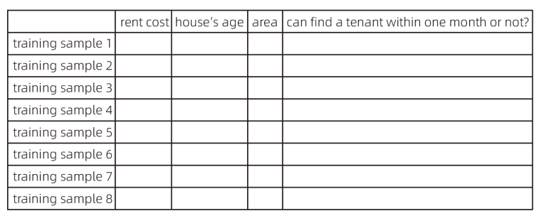
Suppose we need to build a rental analysis model for a specific region. X1, X2, and X3 represent the house’s age, area, and rent, respectively. The goal is to analyze whether a property can find a tenant within one month.

Here, the true value is set as follows: if a tenant is found, the true value is 1; if no tenant is found, the true value is 0.

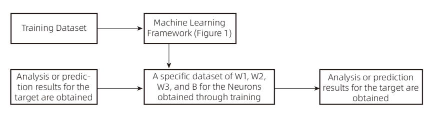
First, we need to prepare training samples and use historical rental data to train the model based on the architecture in Figure 1. The output value is compared with the true value to calculate the deviation. Backpropagation is then used to adjust the parameters, ultimately obtaining a final parameter set (where the deviation between the output and true value is minimized or near the minimum). Subsequently, the data to be analyzed is computed with the final parameter set to obtain the result (analysis outcome). In theory, the closer the output is to 1, the higher the likelihood of finding a tenant within one month; the closer it is to 0, the lower the likelihood.

The above example illustrates a very simple case in deep learning, where features are still manually defined, organized, and quantified, which seems to contradict the earlier statement that “deep learning does not require manual feature setting.” However, in tasks like image recognition, autonomous driving, or video generation, explicit feature quantities cannot be obtained.

(Reference: 《人人可懂的深度学习》，ISBN：9787111680109)

(Reference: 《人人可懂的深度学习》，ISBN：9787111680109)

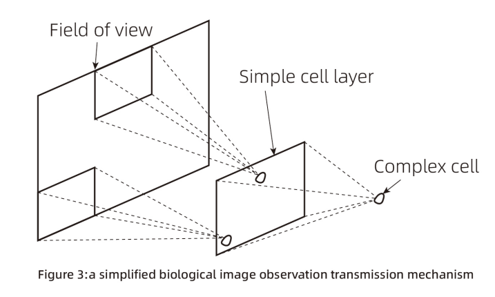
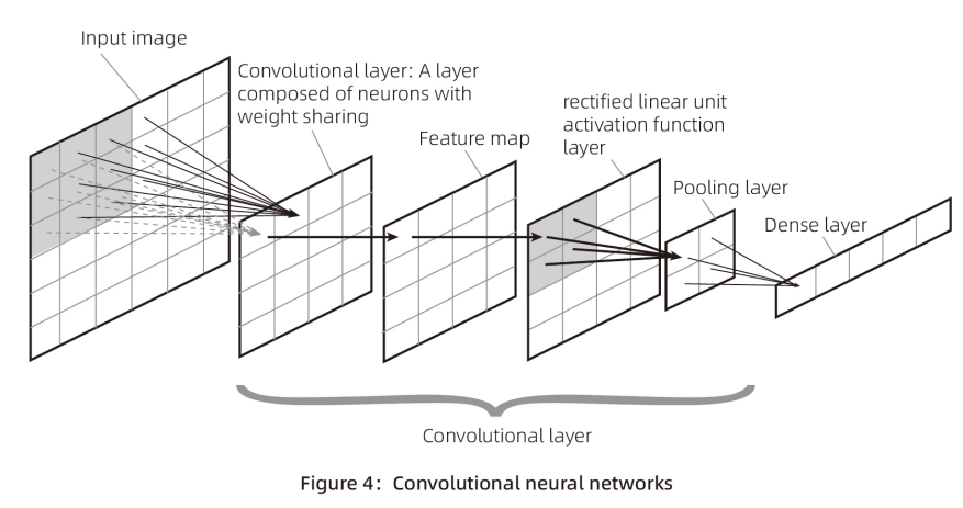
Figure 3 presents a simplified biological image observation transmission mechanism, which is similar to the convolutional neural network scheme in Figure 4. Convolutional neural networks are typically used for image recognition, face recognition, and similar tasks. Their structure differs from Figures 1 and 2 but generally involves obtaining feature quantities at the input layer, assigning weights (setting W and B values) in each neuron to compute output values, introducing an activation function to make the neuron outputs non-linear, and iterating this process multiple times to obtain a specific form of output. After obtaining the output, it is compared with reality to derive a comparison result, and backpropagation is used to adjust the W and B values of each layer, ultimately obtaining a satisfactory parameter set (a collection of W and B values).

In the application scenarios of Figure 4 (likely image-related), unlike the rental data example, there is no logically clear feature quantity data. Each pixel in an image (represented by three values for red, yellow, and blue) is processed through convolutional layers to generate a feature map (feature quantities). Convolutional neural networks apply a process akin to sliding window scanning of image data (three-color data) in the convolutional layer, typically without requiring manual intervention to define image feature variables.

Of course, the above is an extremely simplified overview. Deep learning schemes are diverse and ever-changing, and this book does not intend to cover them exhaustively or analyze their principles in detail. Through the examples in Figures 1, 2, 3, and 4, the diversity and basic structure of AI schemes are illustrated. Given the book’s writing goals, to make the subsequent content more accessible, deep learning is introduced only briefly, and this simplification may involve some inaccuracies. Readers seeking a precise understanding of this technology should refer to professional books.